A Visual Tour¶

Some ideas land faster as a picture than a paragraph. This page is for visual learners: it gathers diagrams of how the pieces fit together, plots that make the maths tangible, photographs from the field, and videos to watch. Everything here is cross-linked to the chapter where you can dig in.

How it all fits together¶

These diagrams render live in your browser (Mermaid), so they stay crisp at any zoom.

The radio signal chain¶

From a faint cosmic whisper to a number on your screen — the path every radio telescope shares.

flowchart LR
  Sky[Cosmic radio source] --> Feed[Antenna + feed horn]
  Feed --> LNA[Low-noise amplifier]
  LNA --> Filter[Band-pass filter]
  Filter --> RX[Receiver / SDR]
  RX --> ADC[Digitiser - ADC]
  ADC --> PC[Computer]
  PC --> Sci[Spectra · images · science]

The amplifier comes first because it sets the noise floor; the filter tames strong out-of-band signals that would swamp an 8-bit SDR. See Chapter 4 and Chapter 5.

The interferometry & imaging pipeline¶

How an array of dishes becomes an image — the subject of Chapters 7–9.

flowchart LR
  A1[Antenna 1] --> C[Correlator]
  A2[Antenna 2] --> C
  An[Antenna N] --> C
  C --> V["Visibilities V(u,v)"]
  V --> Cal[Calibration]
  Cal --> FT[Inverse Fourier transform]
  FT --> DI[Dirty image]
  DI --> CLEAN[CLEAN deconvolution]
  CLEAN --> Img[Science image]

The CLEAN loop¶

Högbom's algorithm (Chapter 9), as a flowchart.

flowchart TD
  Start([Dirty image + dirty beam]) --> Peak[Find brightest pixel]
  Peak --> Sub[Subtract gain x shifted dirty beam]
  Sub --> Rec[Record a clean component]
  Rec --> Check{Peak below threshold,<br/>or max iterations?}
  Check -- no --> Peak
  Check -- yes --> Restore[Convolve components with clean beam,<br/>add residual]
  Restore --> Done([Restored science image])

From the hydrogen line to dark matter¶

The logical chain behind Chapter 11.

flowchart LR
  HI["HI 21 cm emission"] --> Dop[Doppler-shifted velocities]
  Dop --> RC["Rotation curve v(R)"]
  RC --> Flat{Curve stays flat<br/>at large R?}
  Flat -- yes --> DM[Unseen mass → dark matter]
  Flat -- Keplerian falloff --> Lum[Mass traces light]

The maths, made visual¶

These figures are generated from the jansky helper package by scripts/generate_figures.py (Seaborn + the same code the chapters use), so they stay honest to the equations.

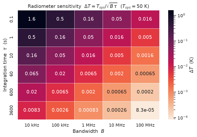
The radiometer equation, as a heatmap¶

Sensitivity improves as \(\sqrt{B\,\tau}\) — more bandwidth and more time both help. Read off how faint a signal you can reach. (Chapter 3)

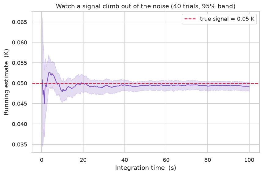
Radiometer sensitivity heatmap over bandwidth and integration time

Watching a signal climb out of the noise¶

Forty simulated integrations (95% band) converging on a faint 0.05 K source as you integrate down. (Chapter 3)

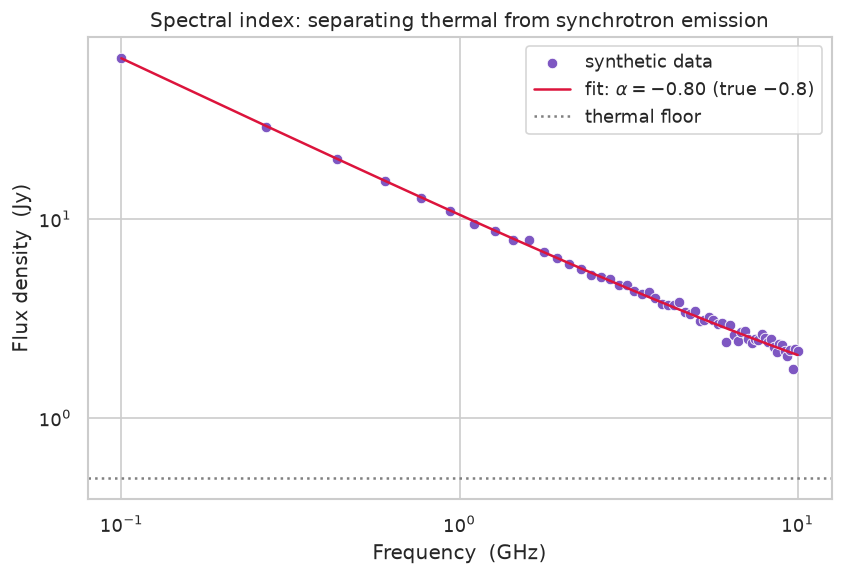
Running estimate converging on a faint signal

Spectral index: thermal vs synchrotron¶

A two-component radio spectrum on log–log axes, with the power-law index recovered by fitting. (Chapter 2)

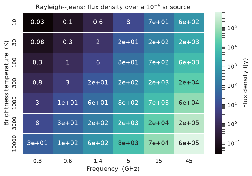
Two-component radio spectrum with fitted spectral index

Brightness temperature → flux density¶

The Rayleigh–Jeans law made tangible: how kelvin map to janskys across the radio band. (Chapter 2)

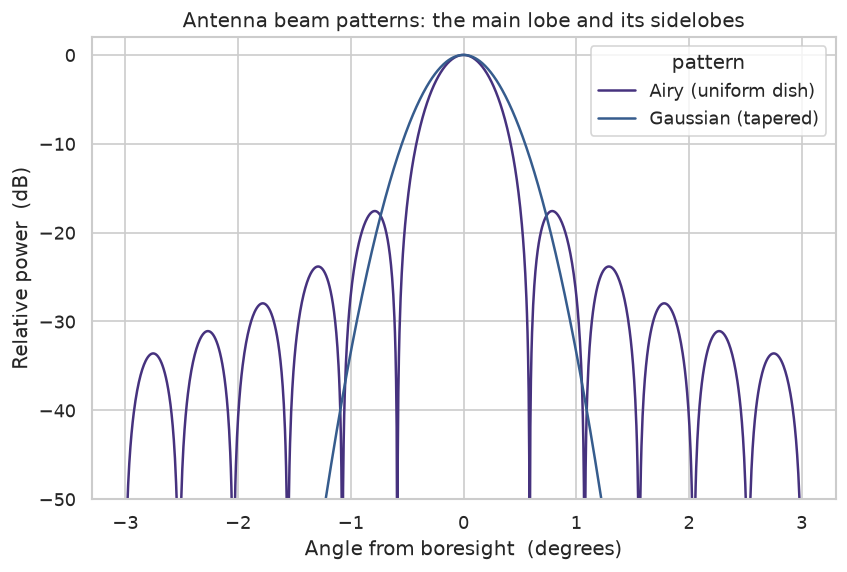
Flux density heatmap over brightness temperature and frequency

Antenna beam patterns¶

The main lobe and its sidelobes for a uniform dish (Airy) vs a tapered (Gaussian) illumination, in decibels. (Chapter 4)

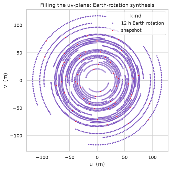
Airy and Gaussian beam patterns in decibels

Filling the uv-plane¶

Why a snapshot isn't enough: Earth rotation sweeps each baseline into an arc, filling the Fourier plane. (Chapter 8)

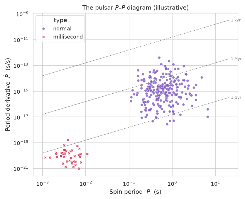
Snapshot versus Earth-rotation uv coverage

The pulsar P–Ṗ diagram¶

The radio astronomer's "HR diagram": spin period vs its derivative, with characteristic-age lines. Note the separate millisecond-pulsar population. (Illustrative populations.) (Chapter 13)

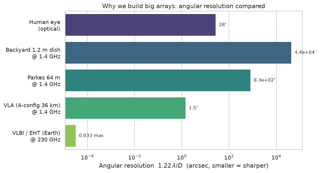
Illustrative pulsar period vs period-derivative diagram

Infographic: why we build big arrays¶

Angular resolution scales as \(1.22\,\lambda/D\) — so a planet-sized array (VLBI/EHT) sees a million times finer than a backyard dish.

Angular resolution compared across instruments

Pictures from the field¶

A short photographic history, from a backyard in the 1930s to a planet-sized telescope. All images are public domain or Creative Commons; credits below each.

Replica of Karl Jansky's rotating antenna at Green Bank Grote Reber's backyard parabolic dish, 1937

Left: full-size replica of Karl Jansky's rotating "merry-go-round" array (the antenna that started it all), public domain. Right: Grote Reber's 1937 backyard dish, the first parabolic radio telescope (source, public domain).

The Karl G. Jansky Very Large Array, New Mexico ALMA antennas on the Chajnantor plain

Left: the Karl G. Jansky Very Large Array (VLA), New Mexico — John Fowler, CC BY 2.0. Right: ALMA antennas at 5,000 m on Chajnantor — ESO/José Francisco Salgado, CC BY 4.0.

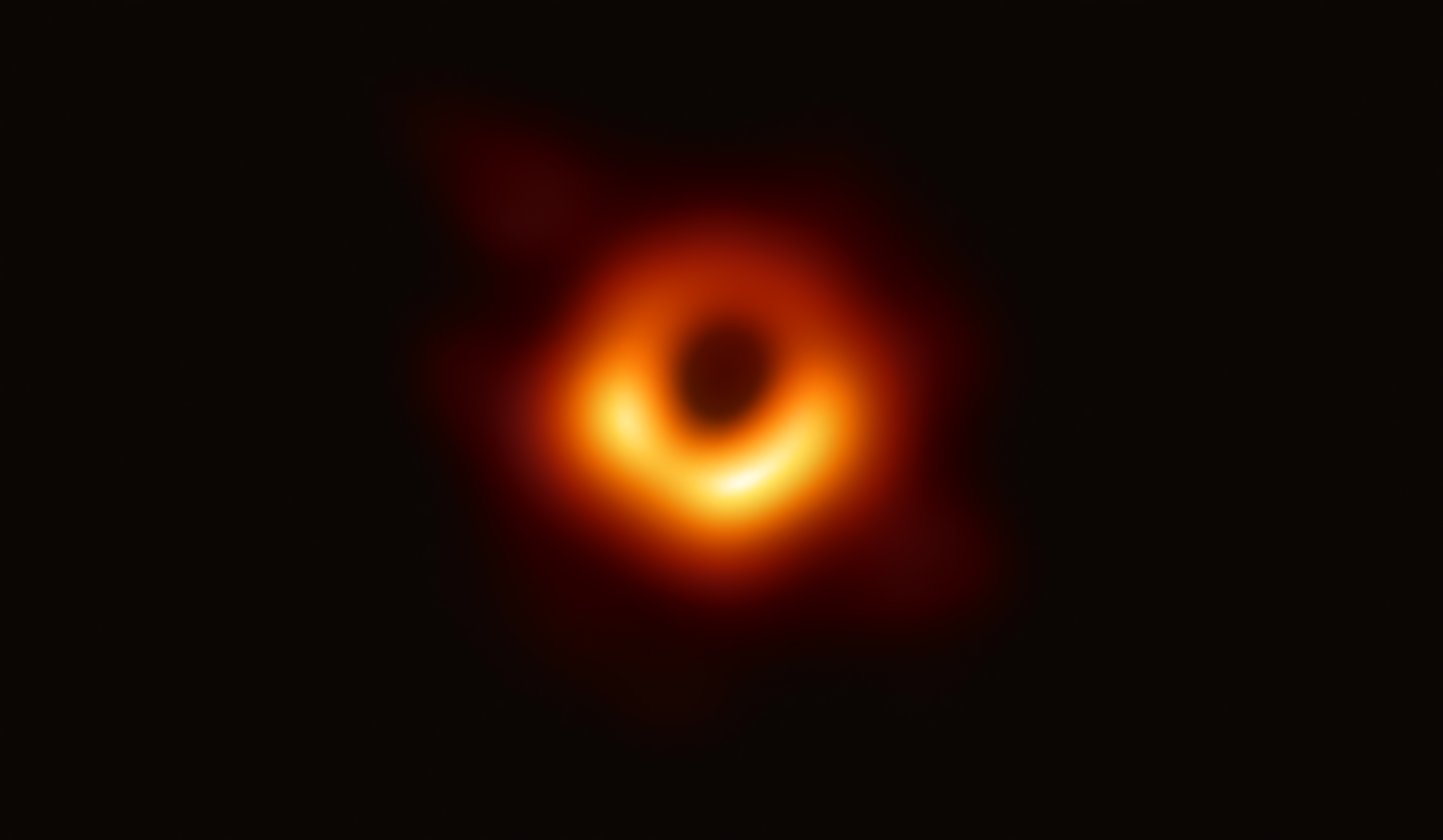
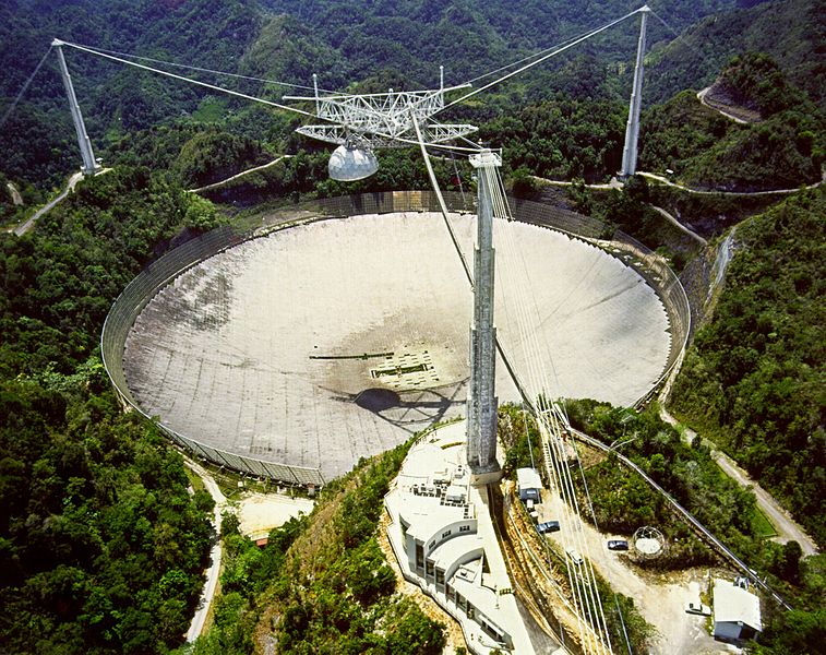
The Event Horizon Telescope image of the M87 black hole Aerial view of the Arecibo Observatory

Left: the Event Horizon Telescope's image of the M87* black hole — assembled by radio interferometry across the planet (EHT Collaboration / ESO, CC BY 4.0). Right: the Arecibo 305 m dish — H. Schweiker/WIYN and NOAO/AURA/NSF, CC BY 4.0.

Cross-section of a satellite LNB feed

A satellite LNB (low-noise block) — the same cheap feed-plus-amplifier hardware amateurs repurpose for hydrogen-line and 11 GHz builds (see Projects). Laurent06, CC BY-SA 3.0.

Watch & learn¶

A hand-picked few to get started — click a thumbnail to watch on YouTube. For the full library of channels and videos organised by topic, see Watch on YouTube.

Foundations¶

Beyond the Visible (NSF/NRAO, narrated by Jodie Foster) — a polished orientation to the VLA and what radio astronomy is for.
Jansky Lecture 1975: The Beginning of Radio Astronomy (NRAO) — Grote Reber, who built the first dish, narrating the field's origins.

Instruments & interferometry¶

Jodrell Bank: the story of the Lovell Telescope — single-dish history and engineering.
How to take a picture of a black hole (Katie Bouman, TED) — the aperture-synthesis pipeline behind the EHT; perfect for Chapters 8–9.

Objects & discoveries¶

The Discovery of Pulsars: A Graduate Student's Tale — Dame Jocelyn Bell Burnell's own account; pairs with Chapter 13.
First Image of a Black Hole (Veritasium) — the result the interferometry chapters build toward.
Pulsar Starquakes Make Fast Radio Bursts? (PBS Space Time) — the FRB frontier.

Build it yourself¶

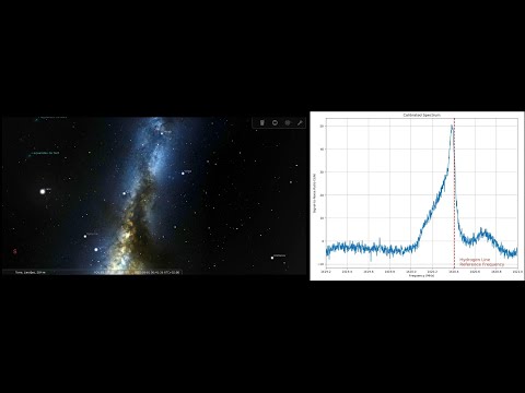
Observing the 21 cm hydrogen line with a DIY radio telescope — a homemade horn + SDR detecting galactic hydrogen; see Projects, Kits & Hacks.

Diagrams and plots in this course are open — regenerate the figures any time with uv run python scripts/generate_figures.py. For the science behind them, follow the chapter links or see the References.